# estimating earth motion with quaternions

This blog is part 1 of me making a very useless device which is a temperature-based clock, telling time by observing the temperature variation over time, and even to a worse accuracy, if specified the latitude, the time of the year. But first I need to model the primary variable source of heat, sun radiation, and that's by first modeling the earth's rotation around its axis and revolution around the sun.

Although the earth's revolution around the sun is set on a plane, the earth's rotation around its axis is rather a very 3D one, and while I can model this motion using linear algebra, that would involve constructing for every motion 3 4x4 matrices for rotation around every axis of the 3D space. A much simpler approach is to use Hamiltonian Quaternions.

First we should note that the binary operation .:H×H->H is not commutative, i.e., the order of applying rotations matters.

To calculate the sun radiation, we should construct two vectors: one from the sun's center to a point p on the earth's surface, which we compute solar radiation for, and another vector, the earth's surface normal at point p. We will consider the variation in longitude very small and we will take the point p of longitude 0. To find the point p, we should rotate a unit vector in the y axis by the latitude angle. Only instead of it being from -90° to 90° with 0° on the equator, it's now from 0° to 180° with 0° being on the north pole. For that, we can utilize the following quaternion: q4 = cos(lat/2) + 0i + sin(lat/2)j + 0k

The first motion we should take note of is the earth's rotation around its axis, which has a constant angular velocity (if we neglect the effect of the moon's tidal friction, which slows it down and stretches the earth's day by about 1.7 milliseconds every century). We can apply the following quaternion after choosing the convention of the z-axis as aligned to the local earth's axis. The time variable is set in terms of days with the 'oneday' variable to tell how many samples we take per day. The angle of the earth at a given hour is given by the following equation: h = ((frame % oneday) / oneday) * 2*pi and the quaternion for this first rotation is q1 = cos(h/2) + 0i + 0j + sin(h/2)k

Then we also need to consider the earth's tilt by 23.44° in the y-axis. The tilt is constant no matter the earth's position around the sun, and it is in world coordinates rather than the earth's, so it should be the last to apply. The tilt in reality does vary by a very negligible amount; for example, it will take 10,000 years to decrease by 1°. The simulation runs over the span of 1 year, so we consider it constant. We apply the following quaternion: 'q3 = cos(tilt/2) + 0i + sin(tilt/2)j + 0k'

Now for the earth's revolution around the sun, we displace the earth by vector R, which we can approximate by a simple uniform rotation, but we won't disappoint Kepler, who demonstrated that planetary movements are elliptic. We first consider an initial linear theta by time: 'theta = (frame2pi)/(365.2oneday)', then we try to solve Kepler's equation 'E − esin(E) = theta'. 5 Newton iterations are probably enough: 'for _ in range(5): E -= (E - esin(E) - theta)/(1 - ecos(E))' 'theta = 2*atan2(sqrt(1+e)sin(E/2), sqrt(1-e)cos(E/2))' The radius from the sun to the earth is 'r = D(1 - ecos(E))' which is a scalar. The vector R is the vector v1 (the initial position of the earth normalized) rotated by the quaternion 'q1 = cos(theta/2) + 0i + 0j + sin(theta/2)k'. Then the earth is displaced by that vector R.

The amount of radiation is easily inferred by calculating the dot product between the vector R and the normal surface vector at the point p, which is the vector from the earth's core to p, the vector (R - p). By neglecting the earth's diameter in comparison to the distance between earth and sun, we can consider the sun's rays as parallel. The only thing left is to prevent the result of the dot product from becoming negative, meaning the surface normal is facing the other side. It doesn't matter which face is the front since it's just a 180° phase longitude shift we already consider unimportant as long as it's consistent. If the result is negative, it will be set to 0.

Note: the synodic day or solar day is slightly longer than 24 hours. That's why there is a slight shift in where the day starts and ends on the data. The earth has 365 solar days; 1 solar day is added since the earth has rotated around the sun. That leaves the earth with 364 rotations around its axis. To correct that effect, simply use i_solar = i - i/365.2 = i*0.9972. This is yet another approximation; the length of the day varies throughout the year.

this is a daily snapshot of the solar radiation in exactly 12h00 UTC everyday of the year.

the anual average solar radiation:

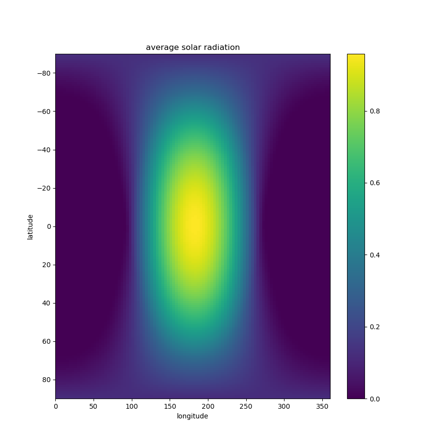
we can see that they are on the daily level just Bell curves with variying lambdas and mus

python code for the computation and animation on blender

TODO: rewrite in haskell

import bpy
from mathutils import Quaternion, Vector
from math import radians, sin, cos, pi, sqrt, tan, atan2

tip = bpy.data.objects.new("VectorTip", None)
bpy.context.collection.objects.link(tip)

# Original vector
D = 5
d = 1
v1 = Vector((1, 0, 0))
v2 = Vector((0, 0, 1))

# Store trajectory points
points = []
datt = []

obj = bpy.context.active_object
obj.rotation_mode = 'QUATERNION'

for frame in range(36525):

    # every 100 frame is one day
    oneday = 100
    theta = (frame*2*pi)/(365.2*oneday)
    M = theta
    e = 0.0167
    E = M
    for _ in range(5):
        E -= (E - e*sin(E) - M)/(1 - e*cos(E))

    theta = 2*atan2(
        sqrt(1+e)*sin(E/2),
        sqrt(1-e)*cos(E/2)
    )

    r = D*(1 - e*cos(E))

    hours = ((frame%oneday)/oneday)*2*pi
    tilt = radians(23.44)

    q1 = Quaternion((cos(theta/2), 0, 0, sin(theta/2)))
    q2 = Quaternion((cos(hours/2), 0, 0, sin(hours/2)))
    q3 = Quaternion((cos(tilt/2), 0, sin(tilt/2), 0))
    R = r * q1 @ v1
    solar_dir = -R.normalized()
    dat = []

    for i in range(181):
        lat = radians(i)
        q4 = Quaternion((cos(lat/2), 0, sin(lat/2), 0))
        n =  q3 @ q2 @ q4 @ v2
        p =  R + (d * n)
        dat += [max(solar_dir.dot(n), 0)]
    datt += [dat]
    
    lat = radians(90 - 33)
    q4 = Quaternion((cos(lat/2), 0, sin(lat/2), 0))

    obj.rotation_quaternion = q3 @ q2
    obj.keyframe_insert(
        data_path="rotation_quaternion",
        frame=frame
    )
    obj.location = R
    obj.keyframe_insert(
        data_path="location",
        frame=frame
    )

    points.append(p.copy())

    tip.location = p

    tip.keyframe_insert(
        data_path="location",
        frame=frame
    )

curve_data = bpy.data.curves.new(
    "Trajectory",
    type='CURVE'
)

curve_data.dimensions = '3D'

spline = curve_data.splines.new('POLY')
spline.points.add(len(points)-1)

for i, p in enumerate(points):
    spline.points[i].co = (p.x, p.y, p.z, 1)

curve_obj = bpy.data.objects.new(
    "Trajectory",
    curve_data
)

bpy.context.collection.objects.link(curve_obj)


with open("output.txt", "w") as file:
    print(datt, file=file)

code for ploting computed data

import matplotlib
matplotlib.use("Agg")
import matplotlib.pyplot as plt
import matplotlib.animation as animation
import ast

def date(n):
    m = [0, 30, 58, 89, 119, 150,
         180, 211, 242, 272, 303, 333, 365]
    s = ['', 'January', 'Febrary', 'March', 'Abril',
         'May', 'June', 'July', 'August',
         'September', 'October', 'Novenber', 'December']
    for i in range(1, len(m)):
        if n < m[i]: return str(n - m[i-1] + 1) + ' ' + s[i]


with open("output.txt", "r") as file:
        data = ast.literal_eval(file.read().strip())
        file.close()

fig, ax = plt.subplots()
days = []
summ = [[0] * 101 for _ in range(181)]
for i in [int(i*100 + (i*100/365.2)) for i in range(363)]:
        t = list(zip(*data[i:i+101]))
        day = ax.imshow(t, animated=True,
                extent=[0, 360, 90, -90], aspect='auto')
        title = ax.text(0.5, 1.01, date(i//100),
                transform=ax.transAxes, ha='center', animated=True)
        if i == 50: plt.colorbar(day, ax=ax)
        plt.xlabel("longitude")
        plt.ylabel("latitude")
        days += [[day, title]]
        for j in range(len(t)):
                for k in range(len(t[j])):
                        summ[j][k] += t[j][k]/363


ani = animation.ArtistAnimation(fig, days, interval=50)
ani.save("movie.mp4")
plt.close(fig)

matplotlib.use("TkAgg")
import importlib
importlib.reload(plt)

fig2, ax2 = plt.subplots()
im = ax2.imshow(summ, extent=[0, 360, 90, -90], aspect='auto')
plt.colorbar(im, ax=ax2)
plt.xlabel("longitude")
plt.ylabel("latitude")
plt.title("average solar radiation")
plt.show()